← Back to Blog

Introduction

At the heart of modern machine learning lies the goal of modeling a target unknown data distribution \(p_\text{data}\), which is typically done through maximum likelihood estimation. When \(\textit{tractable}\), this principle approach provides a robust and statistically sound framework for learning probabilistic models. Yet in practice, approximating the likelihood of the complex and high-dimensional data presents great challenges. Although some probabilistic models can preserve likelihood tractability through strong assumptions, such constraints can however limit their expressiveness.

Energy and Likelihood

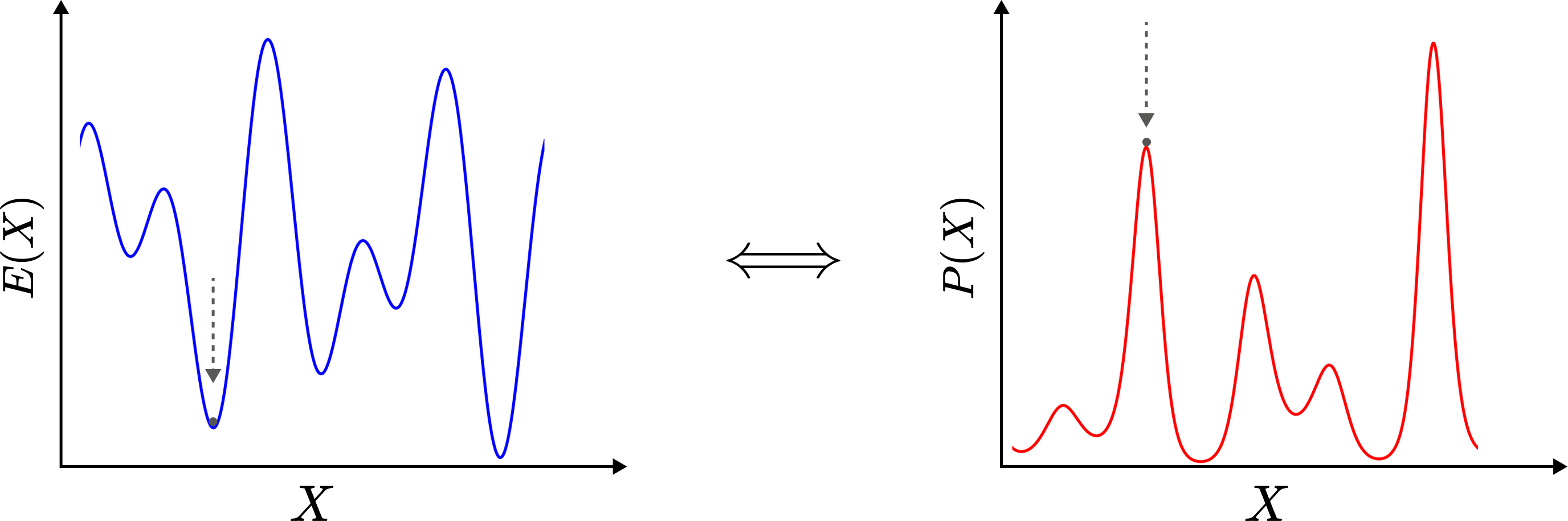
This tension between tractability and expressiveness consequently led to great interests in Energy-based Models (EBMs), as they avoid the requirement of learning a normalized probability density in favor of directly learning an energy function which plays a role in determining the likelihood of the data:

\[p_\theta(x) = \frac{\exp(-E_\theta(x))}{Z_\theta}\]

where \(Z_\theta = \int \exp (-E_\theta(x)) \mathrm{d}x\) is the partition function marginalized over \(x \in \mathbb{R}^N\) and \(\theta\) is a set of learnable parameters.

The goal of learning \(E_\theta (x) : \mathbb{R}^{N} \rightarrow \mathbb{R}\) such that \(p_\theta (x) \approx p_\text{data} (x)\) enables greater flexibility, since EBMs in principle can be defined with any differentiable architecture and trained using gradient-based methods, allowing them to model complex and high dimensional data while avoiding strong constraints, e.g., requiring the model to produce probabilities via \(\texttt{softmax}\).

Although the phrase EBMs may make these models appear niche, it turns out that diffusion models, which are a type of EBMs, have been setting the state-of-the-art performances across a variety of domains and are now the standard when it comes to image and video generations. In much recent times, such models are also experiencing a strong burgeoning interest in language modeling. Although I am biased, due to the fact that I work in this domain, I think EBMs will definitely replace the typical Autoregressive models when it comes to language modeling in the near future (but I will not be making my arguments here).

How to Learn the Energy?

In the typical setup of learning a model \(p_\theta(x) \in [0, 1]^{K}\), where \(\sum_{i}^K p^{(i)}_\theta(x) = 1\) and \(K\) is the number of categories, we heavily rely on the minimization of the negative likelihood to learn our model’s set of parameters \(\theta\):

\[\mathcal{L}(\theta) = - \mathbb{E}_{x \sim p_\text{data}} \big [ \log p_\theta(x) \big ]\]

which is typically accomplished by minimizing the function Cross-Entropy. This means that we would like to constraint our model to produce a set of \(K\) logits which we will then convert to a set of probabilities via the \(\texttt{softmax}\) function. However, as stated above, there is an alternative way to accomplish \(p_\theta (x) \approx p_\text{data} (x)\) without constraining our model to producing a set of probabilities or \(K\) logits.

Specifically, minimizing the negative likelihood of the data is equivalent to minimizing the KL divergence between \(p_\text{data}(x)\) and \(p_\theta(x)\):

\[-\mathbb{E}_{x \sim p_\text{data}(x)} \big [ \log p_\theta (x) \big ] = \mathrm{D}_{KL} \big ( p_\text{data}(x) \, || \, p_\theta (x) \big ) - \mathbb{E}_{x \sim p_\text{data}(x)} \big [ \log p_\text{data} (x) \big ],\]

where \(\mathbb{E}_{x \sim p_\text{data}(x)} \big [ \log p_\text{data} (x) \big ]\) is a constant that does not depend on \(\theta\). As a result, we can estimate the gradient of the log-likelihood:

\[\nabla_\theta \log p_\theta (x) = - \nabla_\theta E_\theta(x) - \nabla_\theta \log Z_\theta.\]

Since \(Z_\theta\) is technically intractable, taking the gradient \(\nabla_\theta \log Z_\theta\) with respect to \(\theta\) enables us to estimate it without worrying about the dependency on \(x\). We can express the second gradient term as the following:

\[\begin{align} \nabla_\theta \log Z_\theta & = \nabla_\theta \log \int \exp \big ( -E_\theta(x) \big ) \mathrm{d} x \\ & = \bigg ( \int \exp \big (-E_\theta (x) \big ) \mathrm{d} x \bigg )^{-1} \bigg ( \nabla_\theta \int \exp \big ( -E_\theta (x) \big ) \mathrm{d} x \bigg ) \\ & = \bigg ( \int \exp \big (-E_\theta (x) \big ) \mathrm{d} x \bigg )^{-1} \int \nabla_\theta \exp \big ( -E_\theta (x) \big ) \mathrm{d} x \\ & = \int \bigg ( \int \exp \big (-E_\theta (x) \big ) \mathrm{d} x \bigg )^{-1} \exp \big ( -E_\theta (x) \big ) \big ( - \nabla_\theta E_\theta (x) \big ) \mathrm{d} x \\ & = \int p_\theta (x) \big ( - \nabla_\theta E_\theta (x) \big ) \big ) \mathrm{d}x \\ & = \mathbb{E}_{x \sim p_\theta (x)} \big [ - \nabla_\theta E_\theta (x) \big ], \end{align}\]

To estimate \(\nabla_\theta \log Z_\theta\), we can obtain an unbiased sample \(x'\) from sampling approaches, such as Monte Carlo Markov Chain (MCMC) techniques, by drawing from our evolving distribution \(p_\theta (x)\):

\[\nabla_\theta \log Z_\theta \simeq -\nabla_\theta E_\theta (x').\]

With an efficient MCMC method like Langevin dynamics, we can easily make use of the score function to draw from \(p_\theta (x)\):

\[\begin{align} \nabla_x \log p_\theta(x) &= - \nabla_x E_\theta (x) - \underset{ = ~ 0}{\underbrace{\nabla_x \log Z_\theta}} \\ & = - \nabla_x E_\theta (x), \end{align}\]

since the term \(\nabla_x \log Z_\theta\) does not depend on \(x\).

Conclusion

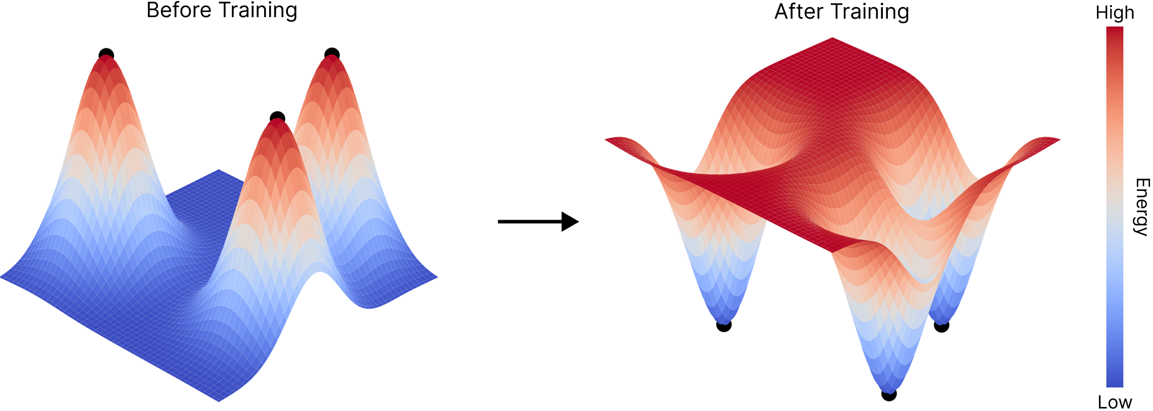
Altogether, the objective (I presented here) is commonly known as Contrastive Divergence, the objective originally utilized to train Boltzmann Machines:

\[\mathcal{L}_{CD}(\theta) = E_\theta(x) - E_\theta(x'),\]

where you take advantage of the model’s (evolving or being learned) distribution and optimize its parameters \(\theta\) by correcting its sampling or generative trajectories with the truth (or data) via enforcing the fact that data points should live on the low-energy positions of the model’s energy landscape while non-data points should live on higher-energy spots.

This intriguing objective \(\mathcal{L}_{CD}\) helps led to the development of much better methods, such as diffusion modeling which arose from score matching, paving the way for modern unsupervised learning.

Finally, a fascinating thing about Enegy-based modeling is its resemblance to Reinforcement Learning. Specifically, both approaches rely on the model’s exploring its learned distribution and make appropriate corrections, to fine-tune its weights (via rewards or simply backpropagate using errors from the truth). However, both approaches only work well if the evolving distribution is relatively accurate and stable, and if the sampling method is accurate enough.

Additional References

1. A Learning Algorithm for Boltzmann Machines. David H. Ackley, Geoffrey E. Hinton, and Terrence J. Sejnowski.
2. How to Train Your Energy-based Models. Yang Song and Diederik P. Kingma.
3. Implicit Generation and Generalization in Energy-Based Models. Yilun Du and Igor Mordatch.
4. Your Classifier is Secretly an Energy Based Model and You Should Treat it Like One. Will Grathwohl, Kuan-Chieh Wang, Jörn-Henrik Jacobsen, David Duvenaud, Mohammad Norouzi, and Kevin Swersky.
5. A Tutorial on Energy-Based Learning. Yann LeCun, Sumit Chopra, Raia Hadsell, Marc’Aurelio Ranzato, and Fu Jie Huang.